Sailboat Playground

Language: EN (complete) / PT-BR (complete)

A simple framework for developing and testing autonomous sailing algorithms with 2D simulations and visualizations.

Getting started

There are two ways to install this package on your machine:

Option #1 - From GitHub repository (recommended)

With this method, you'll be able to run the provided examples without making any changes.

• Clone this repository

https://github.com/gabriel-milan/sailboat-playground

• Navigate to the cloned repository and run

python3 -m pip install .

• And you're done! If you want to run the upwind example, for instance, do

python3 examples/upwind/sailing_upwind.py

Option #2 - From PyPI

This package is also available on PyPI, but you'll need to create your own configuration files for the environment and boat before using it.

• Installing from PyPI:

python3 -m pip install sailboat_playground

Basic usage

This framework is divided into two main modules: engine and visualization.

Engine

The engine module handles the simulation and generates files with simulation data for debugging and later visualization. The main class of the engine is Manager. There, you need to provide both boat and environment configuration files, and optionally, provide data about the boat's orientation, its initial position, and the size of your map (in meters).

An example of usage (explained below) is as follows:

import pickle
from sailboat_playground.engine import Manager

state_list = []
m = Manager(
    "boats/sample_boat.json",
    "environments/playground.json",
    boat_heading=270
)

for step in range(3000):
    state_list.append(m.state)
    state = m.agent_state
    # do stuff here
    m.step([sail_angle, rudder_angle])

with open("out.sbpickle", "wb+") as f:
    pickle.dump(state_list, f)
    f.close()

In the first lines, pickle is imported to serialize the simulation data to a file, and the Manager. Then, a list of states state_list is created, which will be used to store the simulation states.

Next, the Manager is instantiated, passing as arguments two configuration files, one for the boat and one for the environment (to be detailed below) and the initial boat orientation (the convention used is that of the trigonometric circle).

Then, a loop is executed for 3000 iterations. Each iteration corresponds to the time step of the simulator, currently configured for 0.1 seconds. That is, this simulation corresponds to 3000 * 0.1s = 300s = 5 minutes.

Within this loop, the simulation state is stored in state_list. Then, state is assigned the so-called agent_state, which are the environment perceptions from the boat's perspective. The agent_state has the following format:

{
    "heading": xx,
    "wind_speed": xx,
    "wind_direction": xx,
    "position": [xx, xx],
}

where heading corresponds to the sailboat's orientation (the entire coordinate system uses the trigonometric circle convention), wind_speed to the wind speed "felt" by the vessel, wind_direction to the wind direction "felt" by the boat, and position to the boat's position (x,y coordinate). The agent_state can be interpreted as the reading performed by sensors on a real vessel, and only it should be used for developing the autonomous navigation algorithm.

Next, there's a comment do stuff here. It's in this section that the autonomous navigation algorithm logic should be implemented, passing to the Manager only the desired sail and rudder angles in the line m.step([sail_angle, rudder_angle]).

Finally, in the last three lines, this state list is serialized to a *.sbpickle file, to allow later visualization of this simulation.

Visualization

The visualization module only deals with visually demonstrating what happened during the simulation, making it easier to understand and see problems that may exist. The main class of this module is Viewer.

A way to visualize the simulation made in the previous section is as follows (explanations below):

import pickle
from sailboat_playground.visualization import Viewer

with open("output.sbpickle", "rb") as f:
    state_list = pickle.load(f)
    f.close()

v = Viewer()
v.run(state_list=state_list)

In the first two lines we import pickle to deserialize the file we exported in the last section and the Viewer. Then, we load the state_list through the output.sbpickle file.

Next, the Viewer is instantiated. In this case, we don't provide any arguments to it, but it accepts the arguments map_size, for the map size (square, centered at zero, size in meters, default 800 which corresponds to 800m x 800m), and buoy_list, for a list of buoys, in case you want to represent them in the simulation (to demonstrate an IRSC race, for example). The format of the buoy_list should be as follows:

example_buoy_list = [
    (0, 0),     # Buoy positioned at the center of the map
    (-40, -40), # Buoy positioned at coordinate (-40, -40)
]

Finally, in the last line, we run the Viewer passing as argument our state list generated in the simulation. The run method also accepts a simulation_speed argument, which corresponds to the number of timesteps the Viewer will try to execute per second. For example, then, the value 10 would correspond to 10 * 0.1s = 1s per second of visualization (real time). The default value is 100 (10s of simulation per second of visualization). If a very high value is configured, the computer that will execute the instructions may not be able to provide sufficient processing power. In this case, the visualization will be executed at the maximum possible rate.

The visualization has the following format:

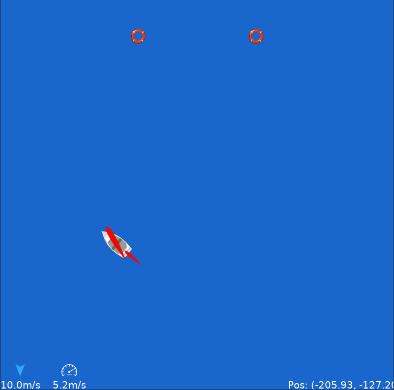
The sailboat is easily identifiable in the image. In the bottom left corner, you can find a blue arrow with a speed below. These are the real wind direction and speed, respectively. Right next to it, a speedometer icon and another value. This is the current speed in magnitude of the sailboat. In the bottom right corner, you can visualize the current position of the sailboat on the map. At the top there are two buoys, to exemplify how they are shown in the visualization. Above the sailboat you can notice two red objects in foil shape. The larger one, in the center of the boat, corresponds to the sail. The smaller one to the rudder. Both the boat and sail and rudder rotate independently, allowing for a more realistic visualization.

Configuration files

To keep the scripts cleaner, all environment configurations (wind speed/direction, variation, gusts, current, etc.) and boat configurations (mass, length, center of mass, foil model, etc.) have been concentrated in separate files in JSON format. In addition, for calculating interaction forces, real lift and drag coefficients extracted from JavaFoil software are used. These coefficients are placed in CSV files.

Environment

An example of environment configuration is as follows (explanations in the example itself):

{
    "name": "Example environment",       // Environment name (no relevance)
    "wind_min_speed": 3,                 // Minimum wind speed (m/s)
    "wind_max_speed": 7,                 // Maximum wind speed (m/s)
    "wind_max_delta_percent": 5,         // Maximum wind variation (percentage) in a timestep
    "wind_gust_probability": 0.1,        // Gust probability (0 to 1 would be 0 to 100%)
    "wind_gust_min_duration": 3,         // Minimum duration of gusts (seconds)
    "wind_gust_max_duration": 20,        // Maximum duration of gusts (seconds)
    "wind_gust_min_speed": 5,            // Minimum wind speed during gust (m/s)
    "wind_gust_max_speed": 10,           // Maximum wind speed during gust (m/s)
    "wind_gust_max_delta_percent": 10,   // Maximum wind speed variation during gust (%)
    "wind_direction": 270,               // Wind direction (degrees), trigonometric circle convention
    "current_speed": 0,                  // Water current speed (m/s)
    "current_direction": 45              // Water current direction (degrees), same convention
}

Boat

An example of boat configuration is as follows (explanations in the example itself):

{
    "name": "Example boat",              // Boat name (no relevance)
    "length": 1.1,                       // Boat length (m)
    "mass": 30,                          // Boat mass (kg)
    "com_length": 0.5,                   // Length from bow to center of mass (m)
    "sail_area": 1.0,                    // Sail area (m^2)
    "sail_foil": "naca0015",             // Sail foil model
    "rudder_area": 0.02,                 // Rudder area (m^2)
    "rudder_foil": "naca0015",           // Rudder foil model
    "hull_area": 0.03,                   // Hull frontal area (m^2)
    "hull_friction_coefficient": 0.2,    // Hull friction coefficient (test experimentally)
    "hull_rotation_resistance": 0.4,     // Hull rotation resistance coefficient (test experimentally)
    "moment_of_inertia": 100             // Boat moment of inertia (test experimentally)
}

Foil model

As it's a foil for more generic purposes (and was used for building the sail of the Glória sailboat), here's a CSV file with the necessary coefficients for the NACA-0015, used in the configuration file above. If you want to insert another foil model, the pattern is a CSV file with three columns: alpha, cl and cd and the lift and drag coefficients for alpha varying from -180 to 180 degrees, with a step of 1 degree.