This project used three datasets with over 72,000 rows of data for movie nominations and winners dating back to 1903.
I completed this project for my Data Science practicum II. I thought it would be a fun project to practice my skills on.
I anlayzed four datasets to complete this project. Two of the datasets were downloaded from www.statcruch.com. The Academy Awards dataset was downloaded from https://www.kaggle.com/theacademy/academy-awards/data.
My project inspiration was to answer the following questions:
- Build a model that predicts the next Oscar winner in any Academy Award category by inputting the nominated movies.
- Determine what variables are significant in predicting an Oscar winning movie?
- Are movie rankings directly correlated to Oscar winning movies?
- Is there a relationship between IMDB rating, number of votes, and Oscar winners?
The three datasets were user friendly and consistantly formated
- Dataset 1: Academy Awards - 8,381 observations and 6 variables
- Dataset 2: Budget/Earnings - 5,222 observations and 7 variables
- Dataset 3: IMDB - 58,786 observations and 25 variables
The fourth dataset was created in R using SQL by bringing together the three above datasets.
- Dataset 4: Combined Dataset - 2,143 observations and 36 variables
Running cluster models was not necesary for this project, because the outliers should not be deleted or ignored.
The outliers where movies that had done particulary well.
I completed this project using R and Tableau. The joining of tables, (GLM) Regression, Random Forest, and a Neuralnet were built within R. The exploratory data was completed in Tableau.
The R Code is located at https://github.com/jenesq/OscarWinner/blob/master/Movie%20R-code.R
The Tableau tables are located at https://public.tableau.com/profile/jenny6450#!/
The Tableau table descriptions are located at https://github.com/jenesq/OscarWinner/blob/master/TableauPublic%20Charts.md
My Oscar presentation is loocated at https://www.youtube.com/watch?v=gDFGiIjSD_w
Data Preparation
I used the following code in order to combine the three datasets and create my final dataset:
data = sqldf("SELECT IMDB.,BudEarn. FROM IMDB
INNER JOIN BudEarn ON IMDB.Title = BudEarn.Movie")
str(data)
data$Movie=NULL
data = sqldf("SELECT data.,Academy. FROM data
INNER JOIN Academy ON data.title = Academy.FilmName")
data$FilmName=NULL
data
Viewing the data:
str(data)
summary(data)
The final data variables in the combined dataset are: movieid, title, year, length, budget, rating, votes, r1, r2, r3, r4, r5, r6, r7, r8, r9, r10, mpaa, action, animation, comedy, drama, documentary, romance, short, month, day, releaseyear, budget($M), domesticGross($M), worldwideGross($M), awardyear, awardceremony, awardtype, awardWinner, awardnomineename.
Exporting dataset to excel to make ensure the inner joins were correct in the SQL script. This dataset was also used in addition to my three downloaded datasets for EDA in Tableau.
write.csv(data, "C:/Users/Jenny Esquibel/Dropbox/Jenny Folder/Data Science Masters/MSDS 696 - Practicum II/CurrentMovieData.xlsx")
Data Cleaning
I quickly realized I had variables that needed to be converted when I looked at the original structure. Below is the code used to convert the variables:
str(data)
data$budget=as.numeric(data$budget)
data$mpaa=as.factor(data$mpaa)
data$Animation=as.factor(data$Animation)
data$Action=as.factor(data$Action)
data$Comedy=as.factor(data$Comedy)
data$Drama=as.factor(data$Drama)
data$Documentary=as.factor(data$Documentary)
data$Romance=as.factor(data$Romance)
data$Short=as.factor(data$Short)
data$AwardWinner=as.factor(data$AwardWinner)
data$Month=as.factor(data$Month)
data$AwardType=as.factor(data$AwardType)
data$releasedate <- with(data, ymd(sprintf('%04d%02d%02d', ReleaseYear, Month, Day)))
data$releasedate
- Checking the data after conversion:
summary(data)
dim(data)
str(data)
Most of the data exploration was performed in Tableau and moved to Tableu Public. All chart descriptions are in the TableauPublic Charts.md file in this project. The direct link to Tableau Public page is https://public.tableau.com/profile/jenny6450#!/.
The charts are also available in the Oscar presentation at https://www.youtube.com/watch?v=gDFGiIjSD_w.
This is one image of the many images created while exploring the data.
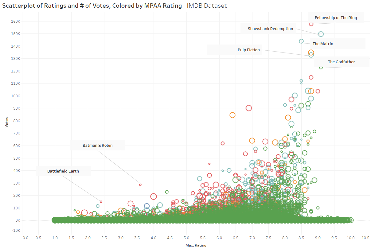
The scatterplot is of movie ratings and number of votes for each movie. The Fellowship of the Ring, Shawshank Redemption, and The Matrix had the most number of votes, but not the highest max ratings.
I needed the following libraries to run my models:
library(sqldf)
library(readxl)
library(lubridate)
library(caTools)
library(caret)
library(MASS)
library(neuralnet)
library(caret)
library(ipred)
Phase 1: (Includes data in all years listed in the dataset)
- Correlation Model
- Step AIC
- GLM Model with AIC
- GLM MOdel without AIC
- Random Forest Model with Grid Search
Phase 2: Includes only the data from 1990 on (Modern Data)
- Correclaton Model with a subet of data for 1990 on
- Step AIC
- GLM Model with AIC
- GLM MOdel withou AIC
- Random Forest Model with Grid Search
- Neural Network
#Subset for 1990 on (finding the modern data only for Phase 2):
dataModern <-subset(data, ReleaseYear >="1990")
str(dataModern)
Phase 1: Looked at all years and used all variables.
#Correlations Matrix (Function borrowed from https://gist.github.com/talegari/b514dbbc651c25e2075d88f31d48057b):
df=data[,c(35,4,5,6,7,18,19,20,21,22,24,26,28,30,33,34,31)]
str(df)
cor2 = function(df){
stopifnot(inherits(df, "data.frame"))
stopifnot(sapply(df, class) %in% c("integer"
, "numeric"
, "factor"
, "character"))
cor_fun <- function(pos_1, pos_2){
#both are numeric
if(class(df[[pos_1]]) %in% c("integer", "numeric") &&
   class(df[[pos_2]]) %in% c("integer", "numeric")){
  r <- stats::cor(df[[pos_1]]
                  , df[[pos_2]]
                  , use = "pairwise.complete.obs"
  )
}

#one is numeric and other is a factor/character
if(class(df[[pos_1]]) %in% c("integer", "numeric") &&
   class(df[[pos_2]]) %in% c("factor", "character")){
  r <- sqrt(
    summary(
      stats::lm(df[[pos_1]] ~ as.factor(df[[pos_2]])))[["r.squared"]])
}

if(class(df[[pos_2]]) %in% c("integer", "numeric") &&
   class(df[[pos_1]]) %in% c("factor", "character")){
  r <- sqrt(
    summary(
      stats::lm(df[[pos_2]] ~ as.factor(df[[pos_1]])))[["r.squared"]])
}

#both are factor/character
if(class(df[[pos_1]]) %in% c("factor", "character") &&
   class(df[[pos_2]]) %in% c("factor", "character")){
  r <- lsr::cramersV(df[[pos_1]], df[[pos_2]], simulate.p.value = TRUE)
}

return(r)
}
cor_fun <- Vectorize(cor_fun)
#now compute corr matrix
corrmat <- outer(1:ncol(df)
, 1:ncol(df)
, function(x, y) cor_fun(x, y)
)
rownames(corrmat) <- colnames(df)
colnames(corrmat) <- colnames(df)
return(corrmat)
}
cor2(df)
-The model tagged the following varaibles as highly correlated:
- Domestic($M) and Worldwid($M) = .967
- Award Ceremony & Award Type = .761
Phase 2: Modern data and used all variables.
#Correlations Matrix (Function borrowed from https://gist.github.com/talegari/b514dbbc651c25e2075d88f31d48057b):
df=dataModern[,c(35,4,5,6,7,18,19,20,21,22,24,26,28,30,33,34,31)]
str(df)
cor2 = function(df){
stopifnot(inherits(df, "data.frame"))
stopifnot(sapply(df, class) %in% c("integer"
, "numeric"
, "factor"
, "character"))
cor_fun <- function(pos_1, pos_2){
#both are numeric
if(class(df[[pos_1]]) %in% c("integer", "numeric") &&
   class(df[[pos_2]]) %in% c("integer", "numeric")){
  r <- stats::cor(df[[pos_1]]
                  , df[[pos_2]]
                  , use = "pairwise.complete.obs"
  )
}

#one is numeric and other is a factor/character
if(class(df[[pos_1]]) %in% c("integer", "numeric") &&
   class(df[[pos_2]]) %in% c("factor", "character")){
  r <- sqrt(
    summary(
      stats::lm(df[[pos_1]] ~ as.factor(df[[pos_2]])))[["r.squared"]])
}

if(class(df[[pos_2]]) %in% c("integer", "numeric") &&
   class(df[[pos_1]]) %in% c("factor", "character")){
  r <- sqrt(
    summary(
      stats::lm(df[[pos_2]] ~ as.factor(df[[pos_1]])))[["r.squared"]])
}

#both are factor/character
if(class(df[[pos_1]]) %in% c("factor", "character") &&
   class(df[[pos_2]]) %in% c("factor", "character")){
  r <- lsr::cramersV(df[[pos_1]], df[[pos_2]], simulate.p.value = TRUE)
}

return(r)
}
cor_fun <- Vectorize(cor_fun)
#now compute corr matrix
corrmat <- outer(1:ncol(df)
, 1:ncol(df)
, function(x, y) cor_fun(x, y)
)
rownames(corrmat) <- colnames(df)
colnames(corrmat) <- colnames(df)
return(corrmat)
}
cor2(df)
The correlation model for the modern dataset flagged the following variables as highly correlated:
- Domestic($M) and Worldwid($M) = .967
- Award Ceremony & Award Type = .761
Phase 1: (Includes data in all years listed in the dataset)
df$AwardWinner=as.numeric(df$AwardWinner)
AICMod <- glm(AwardWinner ~ ., data=df)
modelAward.AIC <- stepAIC(AICMod, direction=c("both"))
modelAward.AIC
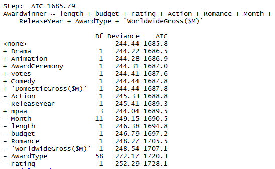
The following 10 variables were selected from the original 17 variables after the Step AIC process:
- AwardWinner, length, budget, rating, action, romance, month, releaseYear, AwardType, worldwideGross($M)
Phase 2: (Modern data)
df$AwardWinner=as.numeric(df$AwardWinner)
AICMod <- glm(AwardWinner ~ ., data=df)
modelAward.AIC <- stepAIC(AICMod, direction=c("both"))
modelAward.AIC
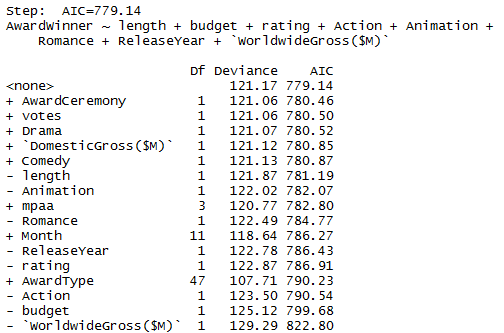
The following 9 variables were selected from the original 17 variables after the Step AIC process:
- AwardWinner, length, budget, rating, action, animation, romance, releaseYear, worldwideGross($M)
Phase 1: All Data
- Running with only the AIC variables:
str(df)
df2=df[,c(1,2,3,4,7,11,12,13,16,17)]
str(df2)
df2$AwardWinner[df2$AwardWinner == "1"] = "0"
df2$AwardWinner[df2$AwardWinner == "2"] = "1"
df2$AwardWinner=as.factor(df2$AwardWinner)
split = sample.split(df2$AwardWinner, SplitRatio = 0.7)
trainset = subset(df2, split == TRUE)
testset = subset(df2, split == FALSE)
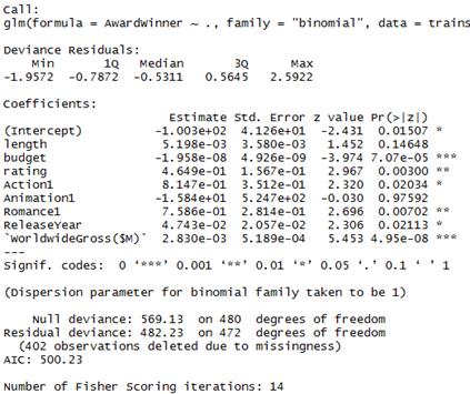
modelAward <- glm(AwardWinner ~ ., data=trainset,family="binomial")
summary(modelAward)
predAward<-predict(modelAward,testset)
predAward2<- ifelse(c(predAward) > 0,1,0)
predictAward3=as.vector(predAward2)
table(testset$AwardWinner, predictAward3)
AccuracyAIC <-(250+54)/(250+54+87+38)
AccuracyAIC
-
Accuracy = .708 ~ 71%
-
Running with all original variables:
df$AwardWinner[df$AwardWinner == "1"] = "0"
df$AwardWinner[df$AwardWinner == "2"] = "1"
df$AwardWinner=as.factor(df$AwardWinner)
split = sample.split(df$AwardWinner, SplitRatio = 0.8)
trainset = subset(df, split == TRUE)
testset = subset(df, split == FALSE)
modelAward <- glm(AwardWinner ~ ., data=trainset,family="binomial")
summary(modelAward)
predAward<-predict(modelAward,testset)
predAward2<- ifelse(c(predAward) > 0,1,0)
predictAward3=as.vector(predAward2)
table(testset$AwardWinner, predictAward3)
AccuracyAIC <-(166+37)/(166+37+65+26)
AccuracyAIC
- Accuracy = .690 ~ 69%
Phase 2: Modern Data
- Running with only the AIC variables:
df$AwardWinner[df$AwardWinner == "1"] = "0"
df$AwardWinner[df$AwardWinner == "2"] = "1"
df$AwardWinner=as.factor(df$AwardWinner)
split = sample.split(df$AwardWinner, SplitRatio = 0.8)
trainset = subset(df, split == TRUE)
testset = subset(df, split == FALSE)
modelAward <- glm(AwardWinner ~ ., data=trainset,family="binomial")
summary(modelAward)
predAward<-predict(modelAward,testset)
predAward2<- ifelse(c(predAward) > 0,1,0)
predictAward3=as.vector(predAward2)
table(testset$AwardWinner, predictAward3)
AccuracyAIC <-(166+37)/(166+37+65+26)
AccuracyAIC
-
Accuracy = .753 ~ 75%
-
Running with all original variables:
- Accuracy = .690 ~ 69%
Phase 1: All Data
Running with all original variables:
df=data[,c(35,4,5,6,7,18,19,20,21,22,24,26,28,30,33,34,31)]
df=na.exclude(df)
df$Domestic=as.vector(df$DomesticGross($M))
df$WorldWide=as.vector(df$WorldwideGross($M))
df$DomesticGross($M)=NULL
df$WorldwideGross($M)=NULL
control <- trainControl(method="repeatedcv", number=10, repeats=3, search="grid")
tunegrid <- expand.grid(.mtry=c(1:15))
rf_gridsearch <- train(as.factor(AwardWinner) ~., data=df, method="rf", tuneGrid=tunegrid, trControl=control)
print(rf_gridsearch)
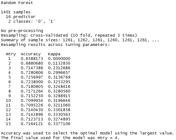
plot(rf_gridsearch)
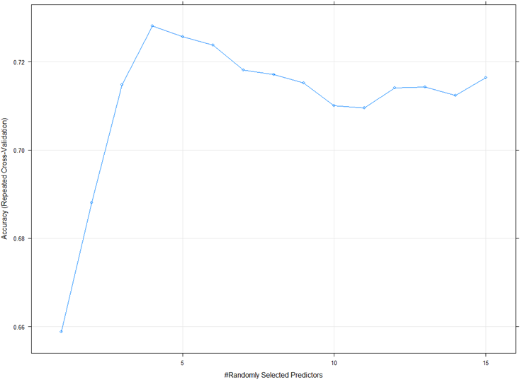
- Accuracy = .728 ~ 73%
Phase 2: Modern Data
Running with all original variables:
df=dataModern[,c(35,4,5,6,7,18,19,20,21,22,24,26,28,30,33,34,31)]
df=na.exclude(df)
df$Domestic=as.vector(df$DomesticGross($M))
df$WorldWide=as.vector(df$WorldwideGross($M))
df$DomesticGross($M)=NULL
df$WorldwideGross($M)=NULL
control <- trainControl(method="repeatedcv", number=10, repeats=3, search="grid")
tunegrid <- expand.grid(.mtry=c(1:15))
rf_gridsearch <- train(as.factor(AwardWinner) ~., data=df, method="rf", tuneGrid=tunegrid, trControl=control)
print(rf_gridsearch)
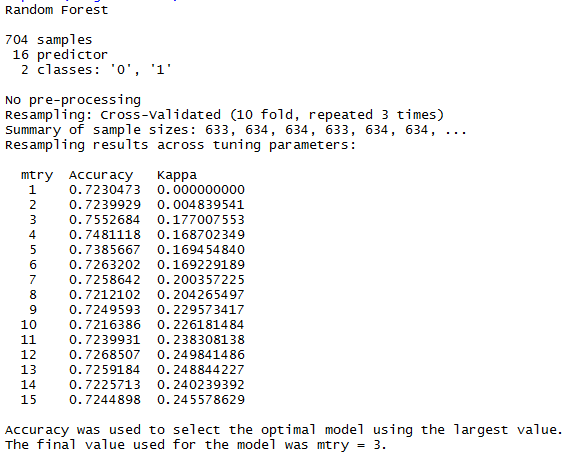
plot(rf_gridsearch)
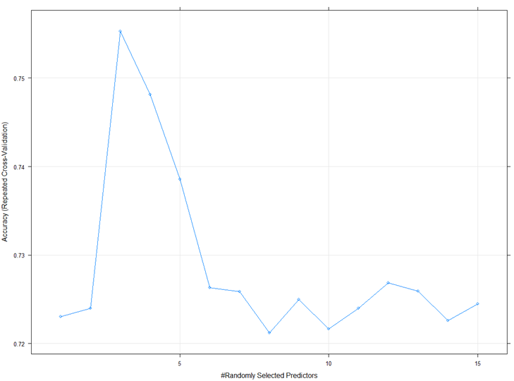
- Accuracy = .755 ~ 76%
Phase 1: All Data
I did not run with all the data.
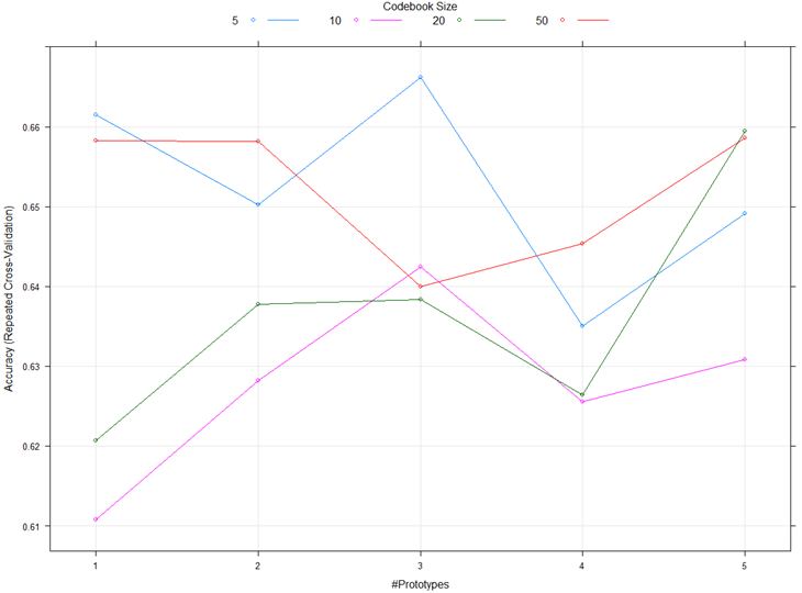
Phase 2: Modern Data
Running with all original variables:
df=dataModern[,c(35,4,5,6,7,18,19,20,21,22,24,26,28,30,33, 34,31)]
df=na.exclude(df)
df$Domestic=as.vector(df$DomesticGross($M))
df$WorldWide=as.vector(df$WorldwideGross($M))
df$DomesticGross($M)=NULL
df$WorldwideGross($M)=NULL
control <- trainControl(method="repeatedcv", number=10, repeats=3, search="grid")
grid <- expand.grid(size=c(5,10,20,50), k=c(1,2,3,4,5))
rf_gridsearch <- train(as.factor(AwardWinner) ~., data=df, method="lvq", tuneGrid=grid, trControl=control, tuneLength=5)
print(rf_gridsearch)
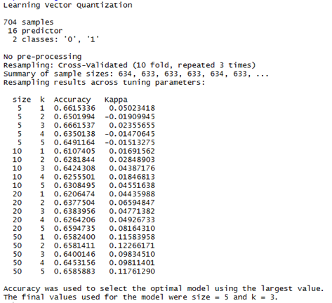
- Accuracy = .660 ~ 66%
plot(rf_gridsearch)
- The best performing prediction model was the Random Forest running with only the Modern data (76%)
- The following variables are significant in predicting an Oscar winning movie:
- AwardWinner, length, budget, rating, action, animation, romance, releaseYear, worldwideGross($M)
- Drama is the genre that wins the most Oscar awards
- Ben-Hur and Titanic each won 10 awards which is the most in Oscar history.
- There is no relationship between IMDB rating, number of votes, and Oscar winners
- For this project a model predicting winners, had a 69% random guessing baseline (no information rate).
- I was able to build models that a higher accuracy rate than random guessing. I am looking forward to running the model on the next nominations.
- The data showed there has been a significant increase in movies being produced each year since 1914 (slide 37, 38, 39).
- Interestingly, there is not a strong correlation between nominations and wins.
- No matter what film wins the awards going to the movies is a great time!
Thank you!
Github.com (2018). Awards. Retrieved from https://gist.github.com/talegari/b514dbbc651c25e2075d88f31d48057b.
Oscars (2018). Oscars. Retrieved from http://www.oscars.org/Oscars.
Wikipedia (2018). Academy Awards. Retrieved from https://en.Wikipedia.org/wiki/AcademyAwards.