Learning Gaussian Splatting

I want to fully grasp 3D Gaussian Splatting. The original code was a bit tough to follow without computer graphics or CUDA background, especially tile-based rendering. So I'm trying my best to implement it from scratch with NumPy and PyTorch, starting with rendering. Simplicity is prioritized over performance.

Core Code Statistics

# tokei camera.py gaussian.py render.py utils.py
├── 📄 camera.py   # Camera model and view transformation utilities
├── 📄 gaussian.py # 3D Gaussian representation and operations
├── 📄 render.py   # Rendering pipeline and projection functions
└── 📄 utils.py    # Helper functions and common utilities

===============================================================================
 Language            Files        Lines         Code     Comments       Blanks
===============================================================================
 Python                  4          662          529           44           89
===============================================================================

Getting Started

Installation

1. Clone the repository:

git clone https://github.com/suous/learn-gaussian-splatting.git
cd learn-gaussian-splatting

2. Install the required dependencies.

uv sync

3. Activate the environment.

source .venv/bin/activate

Data Download

Download the COLMAP and PLY data from Release v1.0.0:

wget -qO-  https://github.com/suous/learn-gaussian-splatting/releases/download/v1.0.0/data.tgz  | tar xz -C .

This will create a data directory with the following structure:

data
├── colmap
│   ├── images
│   │   ├── 000000.png
│   │   ├── ..........
│   │   └── 000024.png
│   └── sparse
│       └── 0
│           ├── cameras.bin
│           ├── images.bin
│           ├── points3D.bin
│           └── points3D.ply
└── point_cloud.ply

# python gaussian.py
==================================================
          Gaussian Splatting Statistics
==================================================

    🎯 Positions  : (37942, 3)
    🔄 Rotations  : (37942, 4)
    📏 Scalings   : (37942, 3)
    💫 Opacities  : (37942, 1)
    🎨 Features   : (37942, 3, 16)
    📊 Covariances: (37942, 3, 3)
    
--------------------------------------------------
Total Gaussians: 37,942
SH Degree      : 3
==================================================

Usage

• Render an Image

python main.py --image_number 0

This will display the original image and the rendered image using matplotlib.

• Generate animation

python main.py --generate_animation

ffmpeg -framerate 8 -pattern_type glob -i "*.png" -vf "fps=10,scale=640:-1,split[s0][s1];[s0]palettegen[p];[s1][p]paletteuse" -loop 0 animation.gif

Results

Basic Idea of 3D Gaussian Splatting

3D Gaussian Splatting (3DGS) is a novel method for representing and rendering 3D scenes, introduced in the paper "3D Gaussian Splatting for Real-Time Radiance Field Rendering" by Kerbl et al. (2023). It has gained significant attention as an alternative to Neural Radiance Fields (NeRFs) due to its impressive rendering speed and quality.

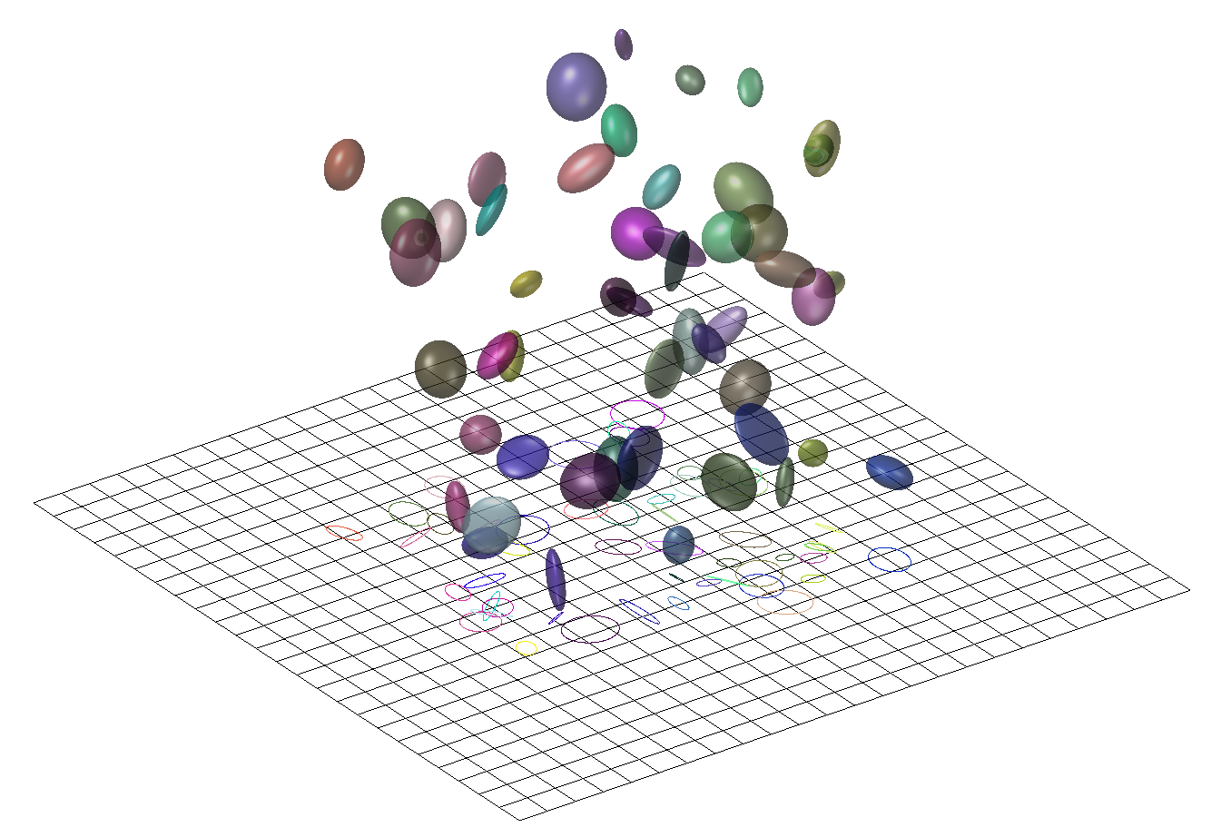
At its core, 3DGS represents a 3D scene as a collection of millions of 3D Gaussians. Each Gaussian is a point in space with specific parameters that define its appearance and shape.

Gaussian Parameters

image from https://3dgstutorial.github.io/3dv_part2.pdf

Each 3D Gaussian is defined by the following parameters:

• Position (Mean $\mu$): A 3D vector representing the center of the Gaussian: $[x, y, z]$.
• Covariance ($\Sigma$): A $3\times3$ matrix that defines the shape, size, and orientation of the Gaussian. To ensure that the covariance matrix remains physically meaningful (positive semi-definite) during optimization, it is decomposed into:
  • Scaling ($S$): A 3D vector representing the scale of the Gaussian along its local axes: $[S_x, S_y, S_z]$.
  • Rotation ($R$): A quaternion representing the orientation of the Gaussian in space: $q=[r, x, y, z]$.
• Color ($c$): The color of the Gaussian, which can be represented as RGB values or, more commonly, as coefficients of Spherical Harmonics (SH) to model view-dependent effects like reflections.
• Opacity ($\alpha$): A value between 0 and 1 that controls the transparency of the Gaussian.

$$ R = \begin{bmatrix} 1 - 2(y^{2} + z^{2}) & 2(xy - rz) & 2(xz + ry) \\ 2(xy + rz) & 1 - 2(x^{2} + z^{2}) & 2(yz - rx) \\ 2(xz - ry) & 2(yz + rx) & 1 - 2(x^{2} + y^{2}) \end{bmatrix} $$

$$\Sigma = RSS^TR^T$$

Rendering

The rendering process in 3DGS is a form of rasterization. For a given camera viewpoint, the 3D Gaussians are projected onto the 2D image plane. These 2D projections are then sorted by depth and blended together, front-to-back, to produce the final color for each pixel.

Mathematical Formulation

The influence of a 3D Gaussian at a point $x$ in space is given by the Gaussian function:

$$ G(x) = e^{-\frac{1}{2}(x-\mu)^T \Sigma^{-1} (x-\mu)} $$

Where:

• $\mu$ is the mean (center) of the Gaussian.
• $\Sigma$ is the covariance matrix.

$$ \Sigma = \begin{bmatrix} \sigma_x^2 & \text{Cov}(x, y) & \text{Cov}(x, z) \\ \text{Cov}(y, x) & \sigma_y^2 & \text{Cov}(y, z) \\ \text{Cov}(z, x) & \text{Cov}(z, y) & \sigma_z^2 \end{bmatrix} $$

During the 3D-to-2D projection process, the Jacobian matrix $J$ represents the derivative of the 2D spatial coordinates $(u, v)$ with respect to the 3D spatial coordinates $(x,y,z)$, i.e.:

$$ J = \frac{\partial (u,v)}{\partial (x,y,z)} = \begin{bmatrix} \frac{\partial u}{\partial x} & \frac{\partial u}{\partial y} & \frac{\partial u}{\partial z} \\ \frac{\partial v}{\partial x} & \frac{\partial v}{\partial y} & \frac{\partial v}{\partial z} \end{bmatrix} $$

3D Gaussian Splatting (3DGS) specifically uses perspective projection. According to the perspective projection formula:

$$ z \begin{bmatrix} u \ v \ 1 \end{bmatrix} = \begin{bmatrix} f_x & 0 & c_x \\ 0 & f_y & c_y \\ 0 & 0 & 1 \end{bmatrix} \cdot \begin{bmatrix} x \ y \ z \end{bmatrix} = z \begin{bmatrix} f_x \frac{x}{z} + c_x \\ f_y \frac{y}{z} + c_y \\ 1 \end{bmatrix} $$

The relationship between $(u,v)$ and $(x,y,z)$ is:

$$ \begin{cases} u = f_x \dfrac{x}{z} + c_x \\ \\ v = f_y \dfrac{y}{z} + c_y \end{cases} $$

The Jacobian matrix $J$ is then derived as:

$$ J = \begin{bmatrix} f_x \dfrac{1}{z} & 0 & -f_x \dfrac{x}{z^2} \\ \\ 0 & f_y \dfrac{1}{z} & -f_y \dfrac{y}{z^2} \end{bmatrix} $$

$$ \Sigma^\prime = JW\Sigma W^TJ^T $$

The final color $C$ of a pixel is computed by blending the projected Gaussians that overlap with it, ordered by depth:

$$ C = \sum_{i \in N} c_i \alpha_i \prod_{j=1}^{i-1}(1 - \alpha_j) $$

Where:

• $N$ is the set of Gaussians overlapping the pixel, sorted by depth.
• $c_i$ is the color of the i-th Gaussian.
• $\alpha_i$ is the final opacity of the i-th Gaussian, which is calculated from its 2D projection.

$$ \alpha_i = \sigma(\alpha_i^\prime) \times e^{-\frac{1}{2}x^T \Sigma_i^{\prime-1} x} $$

• $\alpha^\prime$ is the learned opacity.
• $\Sigma^{\prime}$ is the 2d projection of the 3d covariance.

$$ \Sigma^\prime = \begin{bmatrix} \sigma_x^2 & \text{Cov}(x, y) \\ \text{Cov}(y, x) & \sigma_y^2 \\ \end{bmatrix} $$

Training

The parameters of the Gaussians are optimized to reconstruct a scene from a set of input images with known camera poses. The training process involves:

1. Initialization: The process starts with a sparse point cloud generated from the input images using Structure-from-Motion (SfM), for example, with COLMAP. These points are used to initialize the positions ($\mu$) of the Gaussians.
2. Optimization: The parameters of the Gaussians (position, covariance, color, opacity) are optimized using stochastic gradient descent. The loss function is typically a combination of an L1 loss and a D-SSIM (Structural Dissimilarity Index) term, comparing the rendered images with the training images.
3. Adaptive Densification: During optimization, the set of Gaussians is adaptively modified to better represent the scene. This involves:
   • Cloning: Duplicating small Gaussians in areas that are under-reconstructed.
   • Splitting: Splitting large Gaussians in areas with high variance.
   • Pruning: Removing Gaussians that are nearly transparent (very low opacity).

TODO

• Understand and implement tile based rendering.
• Train from scratch with pytorch code.

References

Papers

• 3D Gaussian Splatting for Real-Time Radiance Field Rendering
• A Survey on 3D Gaussian Splatting
• Mip-Splatting: Alias-free 3D Gaussian Splatting
• 2D Gaussian Splatting for Geometrically Accurate Radiance Fields
• Dynamic 3D Gaussians: Tracking by Persistent Dynamic View Synthesis
• 4D Gaussian Splatting for Real-Time Dynamic Scene Rendering
• VastGaussian: Vast 3D Gaussians for Large Scene Reconstruction

Courses

• Games101
• Visualizing quaternions (4d numbers) with stereographic projection
• 【论文讲解】用点云结合3D高斯构建辐射场，成为快速训练、实时渲染的新SOTA！

Blogs

• 3D Gaussian Splatting Tutorial
• A Comprehensive Overview of Gaussian Splatting
• Introduction to 3D Gaussian Splatting
• Exploring 3D Gaussian Splatting
• 3D Gaussian Splatting Introduction – Paper Explanation & Training on Custom Datasets with NeRF Studio Gsplats
• Rendering in 3D Gaussian Splatting
• 3D Gaussian Splatting
• 详解3D Gaussian Splatting CUDA Kernel：前向传播
• 2DGS: 2D Gaussian Splatting for Geometrically Accurate Radiance Fields
• Understanding 3D Gaussian Splats by writing a software renderer
• [Concept summary] 3D Gaussian and 2D projection

Code

• 3dgs-warp-scratch
• torch-splatting

❤️ Thanks to Cursor for generating well-formatted code comments!