MSDS 692 Barley Marker Validation Project
Barley is a key ingredient in brewing beer. It is also an important cereal grain that provides some food to humans, but mostly to livestock. I work for a large beer company breeding barley. Our goal is to improve the barley varieties available to brewers and farmers. The barley needs to produce good beer, but it also needs to be profitable for the farmer. New varieties are slow to produce with a new line taking about 14 years to be commercially grown after first being made. It then takes another one to two years to make it into large scale beer production. With a global environment that is changing, 15 years is a long time and many varieties are abandoned long before making it to market.
In order to help speed up the process, and make it more accurate, genetic assisted selection is starting to be used. This is different from genetically modifying in that the genes are not physically altered by man made processes, instead plants are screened to identify the genes they contain. Only the plants with desirable genes continue through the pipeline. The biggest problem currently is we do not know what genes are associated with what traits. It is quickly being mapped by academics, but they are generally looking at barley that is different from what we have. Academics use many types of barley in their research, like feed barley. From papers and research institutions there are approximately 200 genes associated with traits.
The goal of this project is to validate DNA markers used in barley breeding at my company. The genes are commonly referred to as markers. The markers currently used were determined from looking at barley varieties used by academia. To be useful to the company where I work, the markers need to be correlated to physical traits with our varieties. Basically, we need to see if the markers identified by academia to be associated to certain traits are also associated with those traits in our 'in house' varieties.
Select varieties were screened in 2015. As the breeding process progresses, varieties determined to be less desirable are dropped. The data set has physical observations from 2015, 2016, and 2017, however, 2016 and 2017 do not contain all the varieties that were in 2015. More over, the malt analysis lab did not run tests on varieties. The varieties, for the most part, should be genetically fixed for every trait. This means that every variety should be homozygous for every marker and we will make the assumption that there are only two alleles (choices) for each gene. Barley is diploid, like humans, meaning that there are two of every chromosome which make the genetics much easier because there are less dominance issues. Being homozygous at every marker means that each marker within a given line should have two copies of the same allele. For each marker there should be two populations of varieties, one with one homozygous set of alleles and one with the other homozygous set of alleles.
In addition to the genetic make up of the variety, the environment where it is grown can have a huge impact on the physical characteristics. Years to year, the same field can produce very different barley from the same variety. For this study, each growing location and crop year made up one trial.
The bulk of the analysis to determine if a physical trait was associated with a marker, t-tests were used. For each marker there were two populations, one with alleles "AA" and the other with alleles "BB" for that marker. Genetic testing is extremely accurate, but sometimes errors do occur where the sample cannot be determined. For those instances I used K-nearest neighbor, using physical traits to classify the missing genetic information. Similarly, with lab test sometimes errors occur resulting in "NA" values. For these, I used K-nearest neighbor to imputate the data.
Once I started looking at the data it was apparent that the different trials would need to be comparable. To do this I normalized the data within each trial, for each trait. From the database, there was one file for physical traits measured by the lab, and another file for physical traits measured in the field. For each I normalized the data for each trial and each trait measured for. Here the loop I used for the lab data:
for (i in 1:nrow(trials)) {
  loc_filter <- filter(Line_Use, COOP_LOC_NM == trials[i,])
  loc_traits <- data.frame(TRAIT_NM = unique(loc_filter$TRAIT_NM))
  for (s in 1:nrow(loc_traits)) {
    trait <- filter(loc_filter, TRAIT_NM == loc_traits[s,])
    trait <- na.omit(trait)
    if(is.na(trait[1,4])) next
    one_trait_norm <- as.data.frame(lapply(trait[4], normalize))
    trait$norm_obs <- unlist(one_trait_norm)
    trait$norm_obs <- as.numeric(trait$norm_obs)
    trait_factors <- sapply(trait, is.factor)
    trait[trait_factors] <- lapply(trait[trait_factors], as.character)
    for (t in 1:nrow(trait)) {
      new_entry <- trait[t,]
      LineNormal[nrow(LineNormal)+1,] = list(new_entry$dbo_LINE_LINE_ID, new_entry$TRAIT_NM, new_entry$OBSRV_NT_NBR, new_entry$OBSRV_EFF_TSP, new_entry$COOP_LOC_NM, new_entry$norm_obs)
    }
  }
}```

Here is the loop for the field data (called plot here):
```R
for (i in 1:nrow(trials)) {
  loc_filter <- filter(Plot_Use, COOP_LOC_NM == trials[i,])
  loc_traits <- data.frame(TRAIT_NM = unique(loc_filter$TRAIT_NM))
  for (s in 1:nrow(loc_traits)) {
    trait <- filter(loc_filter, TRAIT_NM == loc_traits[s,])
    trait <- na.omit(trait)
    if(is.na(trait[1,5])) next
    one_trait_norm <- as.data.frame(lapply(trait[5], normalize))
    trait$norm_obs <- unlist(one_trait_norm)
    trait$norm_obs <- as.numeric(trait$norm_obs)
    trait_factors <- sapply(trait, is.factor)
    trait[trait_factors] <- lapply(trait[trait_factors], as.character)
    for (t in 1:nrow(trait)) {
      new_entry <- trait[t,]
      PlotNormal[nrow(PlotNormal)+1,] = list(new_entry$dbo_LINE_LINE_ID, new_entry$TRAIT_NM, new_entry$OBSRV_NT_NBR, new_entry$OBSRV_EFF_TSP, new_entry$COOP_LOC_NM, new_entry$norm_obs)
    }
  }
}
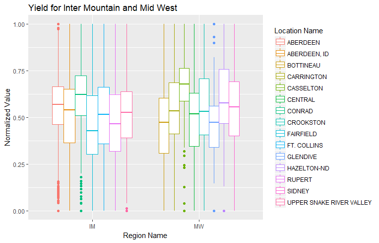
To get an idea of what was going on I looked at yield in the United States. There is an Inter Mountain (IM) region and a Mid West (MW) region:
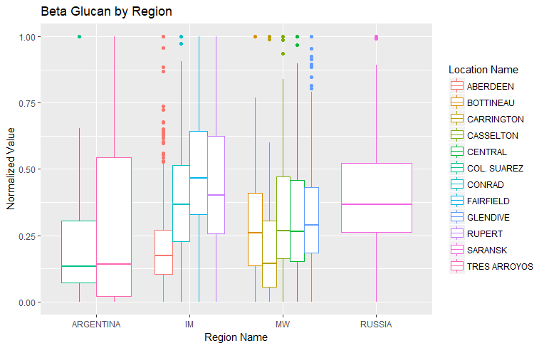
To look at a broader geographical area, I looked at beta glucan across all regions:
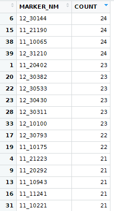
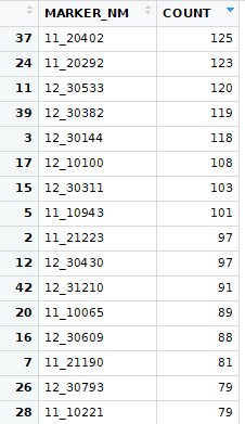
First, I ran t-tests where I compiled the normalized values from every trial for each marker and trait. I then divided them into two groups based on marker allele (HAP_CALL). For each marker and trait I then ran a t-test. This resulted in way too much being significant. Here are the markers with the highest count of significant p-values from the first try:
I also tried a Wilcox text, but that did not look much better:
Then I looked at running t-tests for every trait within each trial:
While these counts appear high, when you take into account the number of trials it ends up looking like this:
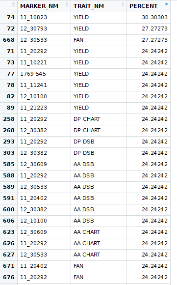
This starts to look better, but is still showing too much is significant, but nothing is significant at a high percent of trials. This is when I shifted to looking at breaking each trial up based on the marker alleles and then finding the average of the sub-populations. Then use those sub-population averages as a sample for the t-test. I determined that the reason for so much appearing significant was the degrees of freedom for each t-test was very high. To reduce the degrees of freedom, I averaged the each trait for each marker type. This kept the original distribution while decreasing the degrees of freedom.
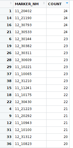
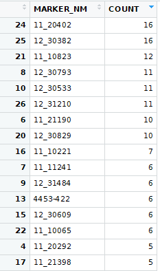
That resulted in markers with significant counts like this:
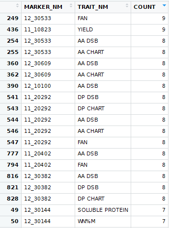
Once again, I drilled down to looking at each trial and I finally got it down to sub-sets for each marker for each trait of each trial. The significant count looked like this:
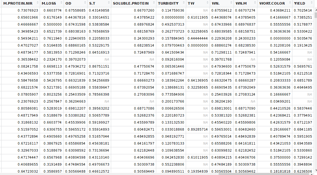
To run the k-nearest neighbor machine learning I partially transformed the data. For each variety at each trial, I created a column for each trait. The resulting table looked like this (there are some middle columns missing):
This is where the lab not having results for every trial became a problem. The table was sparsely populated enough that KNN did not work. I filtered out all the trials that the lab did not run and I got a data frame that was compatible with KNN. I also had to select only columns that had measured values when running the KNN. That table looked like this:
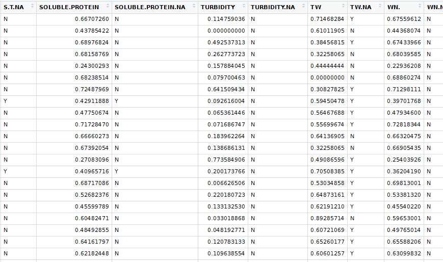
Before running the KNN imputations I created a new table that marked where the missing values were. Then I ran the knnImputation function in the DMwR package. The resulting table looked like this:
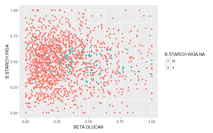
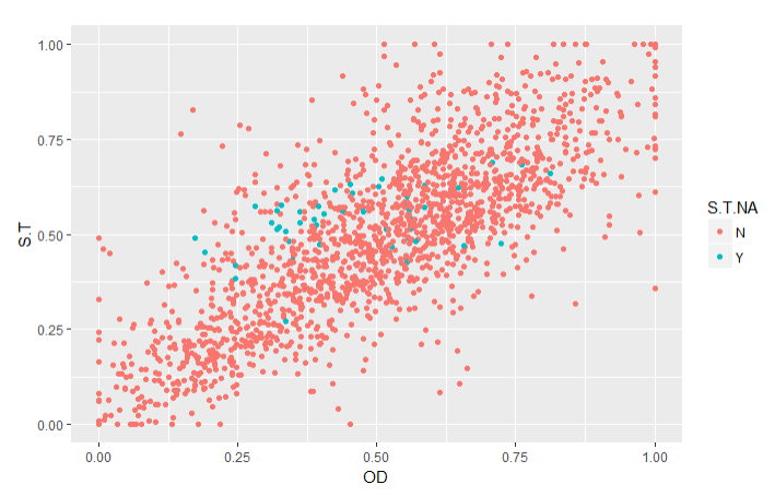
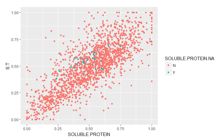
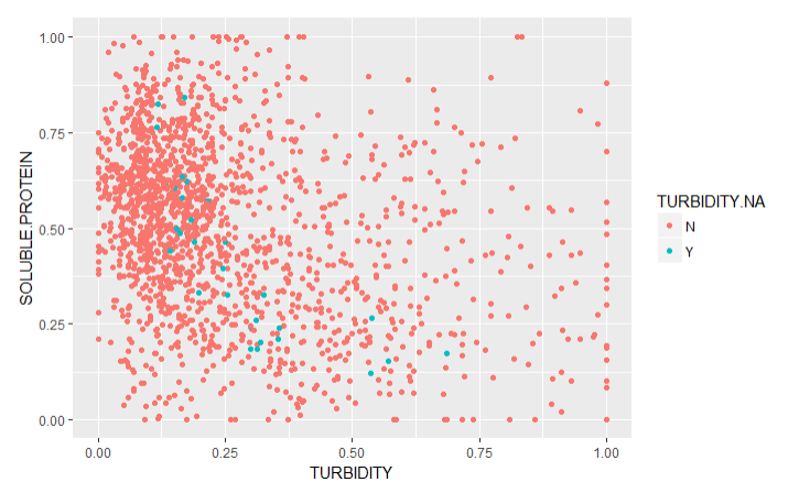
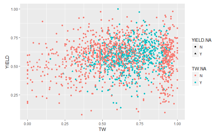
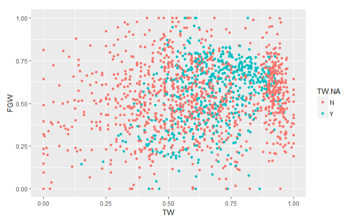
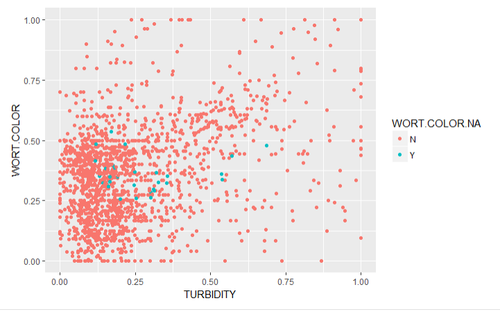
To validate the imputations, I created graphs of the traits with imputed values (Imputed values in blue):
From this chart it is apparent that many of the imputed values were imputed for the same varieties.
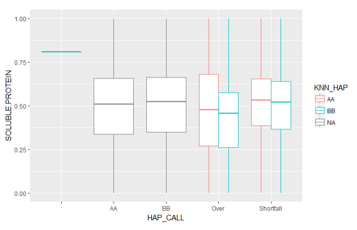
After the imputations, I ran KNN for the classification of genetic markers that did not have an allele value. There were two main types of problem with the genetic data, either the signal was too strong (Over) or two week (Shortfall). KNN was run for every trait in the machine learning dataset (ML_Imputed). A basic boxplot for HAP_CALL vs Soluble Protein shows how close the KNN is :
The main focus of this project was to determine if the markers associated with traits by academia also correlate with traits within our private varieties. The results are decidedly mixed. Of the top 20 markers identified with traits in this study, 11 correlate with the academic materials. While the percentage of this is not very high, the fact that many characteristics originally presented as significant, and even after narrowing the scope, over half correlated shows there is potential for this technology. The more data, and the more complete data that is generated, the more accurate these associations will become.
With regard to KNN machine learning, the knnImputation package was within reason. All the groups of values imputed were clustered within a reasonable range of other values when the corresponding trait was chosen at random. In addition, using KNN to classify missing allele information proved somewhat reliable. The values were not as tightly clustered as some of the imputed values, but they were all in a range that was reasonable to predict what the allele values should be. Machine learning in this application is still going through growing pains, and the more information that it can be fed and learn from, the better it will be in the long term.
Due to the nature of the data I cannot provide all of the data, but I created a small, heavily edited sample of csv files that can hopefully show the basic use of the code.
Link to video: Barley Marker Validation YouTube
